OLI data in fall, 2011（step）

%matplotlib inline
import pandas as pd
import numpy as np
# global configuration: show every rows and cols
pd.set_option('display.max_rows', None)
pd.set_option('max_colwidth',None)
pd.set_option('display.max_columns', None)

1. Data Description

1.1 Column Description

# help_table2: the description for data by steps
df2 = pd.read_csv('OLI_data/help_table2.csv',sep=',',encoding="gbk")
df2 = df2.loc[:, ['Field', 'Annotation']]
df2

	Field	Annotation
0	Row	A row counter.
1	Sample	The sample that includes this step. If you select more than one sample to export, steps that occur in more than one sample will be duplicated in the export.
2	Anon Student ID	The student that performed the step.
3	Problem Hierarchy	The location in the curriculum hierarchy where this step occurs.
4	Problem Name	The name of the problem in which the step occurs.
5	Problem View	The number of times the student encountered the problem so far. This counter increases with each instance of the same problem. Note that problem view increases regardless of whether or not the step was encountered in previous problem views. For example, a step can have a "Problem View" of "3", indicating the problem was viewed three times by this student, but that same step need not have been encountered by that student in all instances of the problem. If this number does not increase as you expect it to, it might be that DataShop has identified similar problems as distinct: two problems with the same "Problem Name" are considered different "problems" by DataShop if the following logged values are not identical: problem name, context, tutor_flag (whether or not the problem or activity is tutored) and "other" field. For more on the logging of these fields, see the description of the "problem" element in the Guide to the Tutor Message Format. For more detail on how problem view is determined, see Determining Problem View.
6	Step Name	Formed by concatenating the "selection" and "action". Also see the glossary entry for "step".
7	Step Start Time	The step start time is determined one of three ways: If it's the first step of the problem, the step start time is the same as the problem start time If it's a subsequent step, then the step start time is the time of the preceding transaction, if that transaction is within 10 minutes. If it's a subsequent step and the elapsed time between the previous transaction and the first transaction of this step is more than 10 minutes, then the step start time is set to null as it's considered an unreliable value. For a visual example, see the Examples page.
8	First Transaction Time	The time of the first transaction toward the step.
9	Correct Transaction Time	The time of the correct attempt toward the step, if there was one.
10	Step End Time	The time of the last transaction toward the step.
11	Step Duration (sec)	The elapsed time of the step in seconds, calculated by adding all of the durations for transactions that were attributed to the step. See the glossary entry for more detail. This column was previously labeled "Assistance Time". It differs from "Assistance Time" in that its values are derived by summing transaction durations, not finding the difference between only two points in time (step start time and the last correct attempt).
12	Correct Step Duration (sec)	The step duration if the first attempt for the step was correct. This might also be described as "reaction time" since it's the duration of time from the previous transaction or problem start event to the correct attempt. See the glossary entry for more detail. This column was previously labeled "Correct Step Time (sec)".
13	Error Step Duration (sec)	The step duration if the first attempt for the step was an error (incorrect attempt or hint request).
14	First Attempt	The tutor's response to the student's first attempt on the step. Example values are "hint", "correct", and "incorrect".
15	Incorrects	Total number of incorrect attempts by the student on the step.
16	Hints	Total number of hints requested by the student for the step.
17	Corrects	Total correct attempts by the student for the step. (Only increases if the step is encountered more than once.)
18	Condition	The name and type of the condition the student is assigned to. In the case of a student assigned to multiple conditions (factors in a factorial design), condition names are separated by a comma and space. This differs from the transaction format, which optionally has "Condition Name" and "Condition Type" columns.
19	KC (model_name)	(Only shown when the "Knowledge Components" option is selected.) Knowledge component(s) associated with the correct performance of this step. In the case of multiple KCs assigned to a single step, KC names are separated by two tildes ("~~").
20	Opportunity (model_name)	(Only shown when the "Knowledge Components" option is selected.) An opportunity is the first chance on a step for a student to demonstrate whether he or she has learned the associated knowledge component. Opportunity number is therefore a count that increases by one each time the student encounters a step with the listed knowledge component. In the case of multiple KCs assigned to a single step, opportunity number values are separated by two tildes ("~~") and are given in the same order as the KC names. Check here to see how opportunity count is computed when Event Type column is present in transaction data.
21	Predicted Error Rate (model_name)	A hypothetical error rate based on the Additive Factor Model (AFM) algorithm. A value of "1" is a prediction that a student's first attempt will be an error (incorrect attempt or hint request); a value of "0" is a prediction that the student's first attempt will be correct. For specifics, see below "Predicted Error Rate" and how it's calculated. In the case of multiple KCs assigned to a single step, Datashop implements a compensatory sum across all of the KCs, thus a single value of predicted error rate is provided (i.e., the same predicted error rate for each KC assigned to a step). For more detail on Datashop's implementation for multi-skilled step, see Model Values page.

1.2 Summarization of Data

This table organizes the data as student-problem-step

df_step =  pd.read_csv('OLI_data/AllData_student_step_2011F.csv',low_memory=False) # sep="\t"
df_step.head(2)

	Row	Sample	Anon Student Id	Problem Hierarchy	Problem Name	Problem View	Step Name	Step Start Time	First Transaction Time	Correct Transaction Time	Step End Time	Step Duration (sec)	Correct Step Duration (sec)	Error Step Duration (sec)	First Attempt	Incorrects	Hints	Corrects	Condition	KC (F2011)	Opportunity (F2011)	Predicted Error Rate (F2011)	KC (Single-KC)	Opportunity (Single-KC)	Predicted Error Rate (Single-KC)	KC (Unique-step)	Opportunity (Unique-step)	Predicted Error Rate (Unique-step)
0	1	All Data	Stu_00b2b35fd027e7891e8a1a527125dd65	sequence Statics, unit Concentrated Forces and Their Effects, module Introduction to Free Body Diagrams	_m2_assess	1	q1_point1i1 UpdateComboBox	2011/9/21 17:35	2011/9/21 17:35	2011/9/21 17:35	2011/9/21 17:35	23.13	23.13	.	correct	0	0	1	.	identify_interaction	1	0.3991	Single-KC	1	0.4373	NaN	NaN	NaN
1	2	All Data	Stu_00b2b35fd027e7891e8a1a527125dd65	sequence Statics, unit Concentrated Forces and Their Effects, module Introduction to Free Body Diagrams	_m2_assess	1	q1_point3i3 UpdateComboBox	2011/9/21 17:35	2011/9/21 17:35	2011/9/21 17:35	2011/9/21 17:35	23.13	23.13	.	correct	0	0	1	.	gravitational_forces	1	0.1665	Single-KC	2	0.4373	NaN	NaN	NaN

2. Data Analysis

df_step.describe()

	Row	Problem View	Incorrects	Hints	Corrects	Predicted Error Rate (F2011)	Opportunity (Single-KC)	Predicted Error Rate (Single-KC)	Opportunity (Unique-step)	Predicted Error Rate (Unique-step)
count	194947.000000	194947.000000	194947.000000	194947.000000	194947.000000	113992.000000	194947.000000	194947.000000	193043.000000	0.0
mean	97474.000000	1.133154	0.379611	0.143172	0.964072	0.237508	419.751066	0.252233	1.035971	NaN
std	56276.495801	0.760515	1.373797	0.852520	0.480346	0.158128	288.365862	0.086406	0.384182	NaN
min	1.000000	1.000000	0.000000	0.000000	0.000000	0.002900	1.000000	0.038600	1.000000	NaN
25%	48737.500000	1.000000	0.000000	0.000000	1.000000	0.117900	171.000000	0.188100	1.000000	NaN
50%	97474.000000	1.000000	0.000000	0.000000	1.000000	0.201400	382.000000	0.240500	1.000000	NaN
75%	146210.500000	1.000000	0.000000	0.000000	1.000000	0.319500	635.000000	0.294700	1.000000	NaN
max	194947.000000	32.000000	413.000000	43.000000	86.000000	0.969300	1410.000000	0.773600	24.000000	NaN

num_total = len(df_step)
num_students = len(df_step['Anon Student Id'].unique())
num_problems = len(df_step['Problem Name'].unique())
num_kcs = len(df_step['KC (F2011)'].unique())
num_null_condition = df_step['Condition'].isnull().sum()  # 空值可不要
print("num_total:",num_total)
print("num_students:",num_students)
print("num_problems:",num_problems)
print("num_kcs:",num_kcs)
print("num_null_condition:",num_null_condition)

n_incorrects = df_step['Incorrects'].sum()
n_hints = df_step['Hints'].sum()
n_corrects = df_step['Corrects'].sum()
print("\n","*"*30,"\n")
print(n_incorrects,n_hints,n_corrects)
print(n_corrects / (n_incorrects + n_hints + n_corrects))

num_total: 194947
num_students: 333
num_problems: 300
num_kcs: 98
num_null_condition: 0

 ******************************

74004 27911 187943
0.6483968011923079

（1）Analysis for Null and Unique value of column attributes

def work_col_analysis(df_work):
    num_nonull_toal = df_work.notnull().sum()  # Not Null
    dict_col_1 = {'col_name':num_nonull_toal.index,'num_nonull':num_nonull_toal.values}
    df_work_col_1 = pd.DataFrame(dict_col_1)

    num_null_toal = df_work.isnull().sum()  # Null
    dict_col_2 = {'col_name':num_null_toal.index,'num_null':num_null_toal.values}
    df_work_col_2 = pd.DataFrame(dict_col_2)

    num_unique_toal = df_work.apply(lambda col: len(col.unique()))   # axis=0
    print(type(num_unique_toal))
    dict_col_3 = {'col_name':num_unique_toal.index,'num_unique':num_unique_toal.values}
    df_work_col_3 = pd.DataFrame(dict_col_3)

    # df_work_col = pd.concat([df_work_col_1, df_work_col_2], axis=1)
    df_work_col = pd.merge(df_work_col_1, df_work_col_2, on=['col_name'])
    df_work_col = pd.merge(df_work_col, df_work_col_3, on=['col_name'])
    return df_work_col
print("-------------------num_unique_toal and num_nonull_toal----------------------")
df_result = work_col_analysis(df_step)
df_result

-------------------num_unique_toal and num_nonull_toal----------------------
<class 'pandas.core.series.Series'>

	col_name	num_nonull	num_null	num_unique
0	Row	194947	0	194947
1	Sample	194947	0	1
2	Anon Student Id	194947	0	333
3	Problem Hierarchy	194947	0	27
4	Problem Name	194947	0	300
5	Problem View	194947	0	32
6	Step Name	194947	0	382
7	Step Start Time	194632	315	33098
8	First Transaction Time	194947	0	34578
9	Correct Transaction Time	182132	12815	33501
10	Step End Time	194947	0	34351
11	Step Duration (sec)	194947	0	2521
12	Correct Step Duration (sec)	194947	0	2187
13	Error Step Duration (sec)	194947	0	2105
14	First Attempt	194947	0	3
15	Incorrects	194947	0	32
16	Hints	194947	0	30
17	Corrects	194947	0	17
18	Condition	194947	0	1
19	KC (F2011)	113992	80955	98
20	Opportunity (F2011)	113992	80955	1206
21	Predicted Error Rate (F2011)	113992	80955	7623
22	KC (Single-KC)	194947	0	1
23	Opportunity (Single-KC)	194947	0	1410
24	Predicted Error Rate (Single-KC)	194947	0	317
25	KC (Unique-step)	193043	1904	1179
26	Opportunity (Unique-step)	193043	1904	25
27	Predicted Error Rate (Unique-step)	0	194947	1

（3）Data Cleaning

Data Cleaning Suggestions

• Redundant columns: Columns that are all NULL or Single value.

• rows that KC (F2011) == null（Do not know the knowledge source）

• rows that Step Start Time == null（This step is too short or more than 10mins, so the data is not reliable）

• Others

df_step_clear = df_step.copy(deep=True) # deep copy

# 直接清除所有”冗余列“
cols = list(df_step.columns.values)
drop_cols = []
for col in cols:
    if len(df_step_clear[col].unique().tolist()) == 1:
        df_step_clear.drop(col,axis =1,inplace=True)
        drop_cols.append(col)

print("the cols num before clear: ",len(df_step.columns.to_list()))
print("the cols num after clear:",len(df_step_clear.columns.to_list()))
for col in drop_cols:
    print("drop:---",col)

the cols num before clear:  28
the cols num after clear: 24
drop:--- Sample
drop:--- Condition
drop:--- KC (Single-KC)
drop:--- Predicted Error Rate (Unique-step)

# Others：'KC (F2011)','Step Start Time' with null value
df_step_clear.dropna(axis=0, how='any', subset=['KC (F2011)','Step Start Time'],inplace = True)

# the remaining columns
print("-------------------num_unique_toal and num_nonull_toal----------------------")
df_result = work_col_analysis(df_step_clear)
df_result

-------------------num_unique_toal and num_nonull_toal----------------------
<class 'pandas.core.series.Series'>

	col_name	num_nonull	num_null	num_unique
0	Row	113817	0	113817
1	Anon Student Id	113817	0	331
2	Problem Hierarchy	113817	0	26
3	Problem Name	113817	0	154
4	Problem View	113817	0	32
5	Step Name	113817	0	240
6	Step Start Time	113817	0	18856
7	First Transaction Time	113817	0	19745
8	Correct Transaction Time	103454	10363	19146
9	Step End Time	113817	0	19623
10	Step Duration (sec)	113817	0	2382
11	Correct Step Duration (sec)	113817	0	2093
12	Error Step Duration (sec)	113817	0	1949
13	First Attempt	113817	0	3
14	Incorrects	113817	0	25
15	Hints	113817	0	25
16	Corrects	113817	0	15
17	KC (F2011)	113817	0	97
18	Opportunity (F2011)	113817	0	1205
19	Predicted Error Rate (F2011)	113817	0	7622
20	Opportunity (Single-KC)	113817	0	1164
21	Predicted Error Rate (Single-KC)	113817	0	315
22	KC (Unique-step)	112869	948	625
23	Opportunity (Unique-step)	112869	948	25

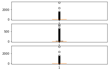
Outlier Analysis

• It is found that there is a non-numeric type in duration that is ‘.’ , which should represent 0

• In addition, box diagrams can be used to analyze whether some outliers need to be removed

print(df_step_clear.columns.tolist())
print("-"*100)
print(df_step_clear.describe().columns.tolist()) #有许多object类无法统计分析
print("-"*100)
print(df_step_clear.dtypes)

['Row', 'Anon Student Id', 'Problem Hierarchy', 'Problem Name', 'Problem View', 'Step Name', 'Step Start Time', 'First Transaction Time', 'Correct Transaction Time', 'Step End Time', 'Step Duration (sec)', 'Correct Step Duration (sec)', 'Error Step Duration (sec)', 'First Attempt', 'Incorrects', 'Hints', 'Corrects', 'KC (F2011)', 'Opportunity (F2011)', 'Predicted Error Rate (F2011)', 'Opportunity (Single-KC)', 'Predicted Error Rate (Single-KC)', 'KC (Unique-step)', 'Opportunity (Unique-step)']
----------------------------------------------------------------------------------------------------
['Row', 'Problem View', 'Incorrects', 'Hints', 'Corrects', 'Predicted Error Rate (F2011)', 'Opportunity (Single-KC)', 'Predicted Error Rate (Single-KC)', 'Opportunity (Unique-step)']
----------------------------------------------------------------------------------------------------
Row                                   int64
Anon Student Id                      object
Problem Hierarchy                    object
Problem Name                         object
Problem View                          int64
Step Name                            object
Step Start Time                      object
First Transaction Time               object
Correct Transaction Time             object
Step End Time                        object
Step Duration (sec)                  object
Correct Step Duration (sec)          object
Error Step Duration (sec)            object
First Attempt                        object
Incorrects                            int64
Hints                                 int64
Corrects                              int64
KC (F2011)                           object
Opportunity (F2011)                  object
Predicted Error Rate (F2011)        float64
Opportunity (Single-KC)               int64
Predicted Error Rate (Single-KC)    float64
KC (Unique-step)                     object
Opportunity (Unique-step)           float64
dtype: object

# Change . to 0 in "xxx-duration"
rectify_cols = ['Step Duration (sec)', 'Correct Step Duration (sec)', 'Error Step Duration (sec)']
for col in rectify_cols:
    df_step_clear[col] = df_step_clear[col].apply(lambda x: 0 if x=='.' else x)
    df_step_clear[col] = df_step_clear[col].astype(float)
print(df_step_clear[rectify_cols].dtypes)

Step Duration (sec)            float64
Correct Step Duration (sec)    float64
Error Step Duration (sec)      float64
dtype: object

3. Data Visualization

import plotly.express as px
from plotly.subplots import make_subplots
import plotly.graph_objs as go
import matplotlib.pyplot as plt
%matplotlib inline

# Outlier analysis for each column

fig=plt.figure()
box_cols = ['Step Duration (sec)', 'Correct Step Duration (sec)','Error Step Duration (sec)']
for i, col in enumerate(box_cols):
    ax=fig.add_subplot(3, 1, i+1)
    ax.boxplot(df_step_clear[df_step_clear[col].notnull()][col].tolist())
fig.show("svg")

D:\MySoftwares\Anaconda\envs\data\lib\site-packages\ipykernel_launcher.py:8: UserWarning:

Matplotlib is currently using module://ipykernel.pylab.backend_inline, which is a non-GUI backend, so cannot show the figure.

# The distribution of continuous values
def show_value_counts_histogram(colname, sort = True):
    # create the bins
    start = int(df_step_clear[colname].min()/10)*10
    end = int(df_step_clear[colname].quantile(q=0.95)/10+1)*10
    step = int((end - start)/20)
    print(start, end, step)
    counts, bins = np.histogram(df_step_clear[colname],bins=range(start, end, step))
    bins = 0.5 * (bins[:-1] + bins[1:])

    fig = px.bar(x=bins, y=counts, labels={'x': colname, 'y':'count'})
    fig.show("svg")


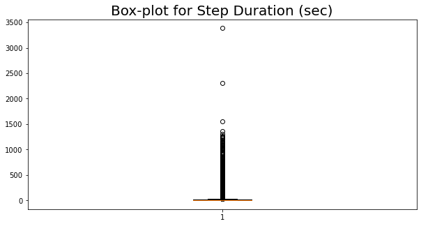
# Box distribution of continuous values
def show_value_counts_box(colname, sort = True):
#     fig = px.box(df_step_clear, y=colname)
#     fig.show("svg")
    plt.figure(figsize=(10,5))
    plt.title('Box-plot for '+ colname,fontsize=20)#标题，并设定字号大小
    plt.boxplot([df_step_clear[colname].tolist()])
    plt.show("svg")


# Histogram of discrete values
def show_value_counts_bar(colname, sort = True):
    ds = df_step_clear[colname].value_counts().reset_index()
    ds.columns = [
        colname,
        'Count'
    ]
    if sort:
        ds = ds.sort_values(by='Count', ascending=False)
    # histogram
    fig = px.bar(
        ds,
        x = colname,
        y = 'Count',
        title = colname + ' distribution'
    )
    fig.show("svg")


# Pie of discrete values
def show_value_counts_pie(colname, sort = True):
    ds = df_step_clear[colname].value_counts().reset_index()
    ds.columns = [
        colname,
        'percent'
    ]
    ds['percent'] /= len(df_step_clear)
    if sort:
        ds = ds.sort_values(by='percent', ascending=False)
    fig = px.pie(
        ds,
        names = colname,
        values = 'percent',
        title = colname+ ' Percentage',
    )
    fig.update_traces(textposition='inside', textinfo='percent+label',showlegend=False)
    fig.show("svg")

# Bar
show_value_counts_bar('First Attempt')
show_value_counts_histogram('Step Duration (sec)')
show_value_counts_box('Step Duration (sec)')

0 70 3

# Pie
# show_value_counts_pie('KC (F2011)')
show_value_counts_pie('Problem Hierarchy')
show_value_counts_pie('Problem Name')
# show_value_counts_pie('Step Name')

# four column labels are individually distributed as follows

topnum_max = 50 # show top 50 for each type
fig = make_subplots(rows=2, cols=2,   # 2*2
      start_cell="top-left",
      subplot_titles=('KC (F2011)','Problem Hierarchy','Problem Name','Step Name'),
      column_widths=[0.5, 0.5])
traces = [
    go.Bar(
        x = df_step[colname].value_counts().reset_index().index.tolist()[:topnum_max],
        y = df_step[colname].value_counts().reset_index()[colname].tolist()[:topnum_max],
        name = 'Type: ' + str(colname),
        text = df_step[colname].value_counts().reset_index()['index'].tolist()[:topnum_max],
        textposition = 'auto',
    ) for colname in ['KC (F2011)','Problem Hierarchy','Problem Name','Step Name']
]
for i in range(len(traces)):
    fig.append_trace(
        traces[i],
        (i //2) + 1, # pos_row
        (i % 2) + 1  # pos_col
    )

fig.update_layout(
    title_text = 'Bar of top 50 distributions for each type ',
)

fig.show("svg")